on Topology

Back in the Saddle

Posted on October 2, 2010 | 1 comment

After Dick Lipton kindly linked my post on hyperspheres, I decided that it was time to maybe get back to blogging. I’ve updated my about page (there’s a tab above too). Check back in the near future, I’ll try to update more often.

1 Comment

Posted in Blog

Geodesics

Posted on July 20, 2009 | Leave a comment

Straight Lines

When we think of a straight line, we usually think of a line in the Euclidean sense; that is, $c(t)=p+tX$ , where $p$ is a point contained in the line, $t$ is a real number, and $X$ is a vector that points parallel to the line. If we consider Euclidean space as a manifold, we would say that $X$ is in the tangent space $T_{c(t)}(\mathbb E^n)$ , because $c'(t)=X$ . One important observation to make is that all along $c(t)$ , $X$ never changes; i.e., we never accelerate. That is, if we move along the curve, we never speed up or slow down, and we never turn.

In the language of my post on covariant derivatives, this is easy to express:

$\nabla_{c'} c' \equiv 0$

The geometric interpretation is simple here: in the direction of the velocity vector, the velocity vector doesn’t change. You can probably see the punchline coming by now. If we generalize to a curve $c(t)$ on a manifold $M$ , $c(t)$ is a geodesic if $\nabla_{c'} c' \equiv 0$ .

Now, you may notice that we can trace out the same curve if we tweak the parameter $t$ so that we could accelerate on the curve (we wouldn’t turn, but we could speed up or slow down). That is, we could have an alternate parametrization. But in order to have a geodesic, we need $\nabla_{c'} c' \equiv 0$ , so $\nabla_{c'}\left<c',c' \right> = 2\left<\nabla_{c'} c',c' \right> = 0$ , and therefore $\|c'\|$ is a constant along the curve. This gives us a unique parametrization of the curve, up to a constant scaling factor on the parameter. In fact, if we consider such a scaling factor, we get that $\nabla_{c'(st)} c'(st) = \nabla_{s c'(t)} s c'(t) = s^2\nabla_{c'(t)} c'(t) = 0$ , so a geodesic with a constant scaling factor on its parameter is still a geodesic (and obviously has the same image). This motivates the following definition: if $\|c'\| = 1$ then the geodesic is called a normal geodesic.

The Exponential Map

Say that some curve $\gamma(t)$ is a geodesic. Then $\nabla_{\gamma'}\gamma' = 0$ is a second-order differential equation in $t$ . If we assume that $\gamma(0) = p$ , and $\gamma'(0) = v$ , then we have the required conditions for existence and uniqueness of a solution to the differential equation. That is, given a point $p\in M$ and tangent vector $v\in T_p(M)$ , there is a unique geodesic $\gamma_v$ that passes through $p$ with velocity $v$ .

The exponential map $\text{exp}_p:T_p(M)\to M$ is defined as $\text{exp}_p(v) = \gamma_v(1)$ , assuming that 1 is in the domain of $\gamma_v$ . The exponential map is fairly important when talking about Riemannian manifolds, and it turns out that it is smooth and a local diffeomorphism. The latter means that there is a neighborhood around $p$ where its unique inverse exists. This inverse is the logarithmic map, or $\text{log}_p:M\to T_p(M)$ .

The exponential map is so important, in fact, that it appears in many of the important theorems in Riemannian geometry, like the Hopf-Rinow Theorem and the Cartan-Hadamard Theorem. It’s also essential to understanding the effects of curvature on a Riemannian manifold.

Arc Length

At this point we can ask about the relationship between arc length and geodesics. Assume that we have some smooth function $\alpha : [a,b]\times(-\epsilon,\epsilon)\to M$ . We can compute the change in arc length $L[c_s]$ over the family of curves $c_s = \alpha | [a,b]\times\{s\}$ :

$\frac d{ds}L[c_s] = \frac d{ds}\int_a^b\left<c_s'(t),c_s'(t)\right>^{1/2}dt = \int_a^b\nabla_S\left<T,T\right>^{1/2}dt$
$= \frac 1 2\int_a^b\left<T,T\right>^{-1/2}\nabla_S\left<T,T\right>dt = \int_a^b\left<T,T\right>^{-1/2}\left<\nabla_S T,T\right>dt$

The variables $S,T$ that we substitute here are fields of tangent vectors corresponding to the differential of $\alpha$ with respect to the variables $s,t$ . The rest is just calculus. Since $s,t$ are independent of each other, we know that their derivatives commute and so we can say that $[T,V] = 0$ . This means that we can make the switch $\nabla_S T = \nabla_T S$ :

$\frac d{ds}L[c_s] = \int_a^b\left<T,T\right>^{-1/2}\left<\nabla_T S,T\right>dt$
$= \int_a^b\left<T,T\right>^{-1/2}\left(T\left<S,T\right>-\left<S,\nabla_T T\right>\right)dt$

If we consider the curve $c_0$ , and consider that we can always reparametrize a curve without loss of generality so that $l = \left<T,T\right>^{1/2}$ is a constant,

$\frac d{ds}L[c_s]\mid_{s = 0} = l^{-1} \left(\left<S,T\right>\mid_a^b-\int_a^b\left<S,\nabla_T T\right>dt\right)$

This is called the first variation formula. The function $\alpha$ is called a variation. If we assume that all the $c_s$ are curves that join two points in $M$ , then we know that $S$ vanishes at the endpoints. If we further assume that $c_0$ is a geodesic, then the integral vanishes (because $\nabla_T T = 0$ ). What this means is that geodesics are critical points of the arc length function $L$ for curves that join two points.

We can’t claim that a geodesic segment minimizes the distance between two points (though there is a unique minimizing geodesic segment; for that we need the second variation formula, which I won’t get into in this post). To see this, consider the case when $M$ is a sphere, with the usual angular metric. If we consider any two distinct points, there is a great circle path that joins them that is of length the angular distance between them, $\delta$ . However, there is also a path of length $2\pi - \delta$ that goes around “the long way” that joins the points as well. This path happens to be the longest one that you can take, and it’s also a geodesic segment. Obviously this would be a maximum of the first variation formula.

It’s easy to see that the first variation formula gives us a lot of power in talking about the geometry of a Riemannian manifold. The source that I use actually motivates the definition of a geodesic from an effort to minimize the first variation formula. I prefer to motivate it from the “straight line” perspective.

Sources

Much of this material comes from Comparison Theorems in Riemannian Geometry by Jeff Cheeger and David G. Ebin.

Leave a comment

Posted in Geometry, Topology

Tagged covariant derivative, differential geometry basics, geodesic, metric

Riemannian Connections

Posted on June 25, 2009 | 2 comments

For the project that I’m working on, I needed to know the basics of riemannian connections. Connections confused the hell out of me until I took a few days to really absorb them. I’m writing down my interpretation here so that I can burn it into the neurons, and hopefully help someone else trying to understand the same topic.

Covariant Derivatives of Scalar Functions

A connection is also called a covariant derivative. One of the principles of differential geometry is that everything should behave the same regardless of which coordinate system you work in, so we’d like a way to get the derivative of a quantity when along an arbitrary direction. When we consider a scalar function f, the covariant derivative is just the directional derivative. If $X = \sum_{k=1}^n b_j E_j$ :

$\nabla_X f = Xf = \sum_{i=1}^n a_i \frac{\partial f}{\partial x_i}$

I found it extremely useful to think of the covariant derivative as a linear operator:

$\nabla_X f = \left(\sum_{i=1}^n a_i \frac\partial{\partial x_i}\right)f$

Covariant Derivatives of Vector Fields

If we want to apply $\nabla_X$ to a vector field $Y$ , then we can apply the operator:

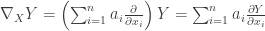
$\nabla_X Y = \left(\sum_{i=1}^n a_i \frac\partial{\partial x_i}\right)Y = \sum_{i=1}^n a_i \frac{\partial Y}{\partial x_i}$

Immediately we can see an interpretation for $\nabla_X Y$ : see how $Y$ changes with respect to each coordinate direction, and then sum the resulting vectors together, weighted by each component of $X$ . It’s easy to see how this gives us a coordinate-free derivative of a vector field. What we have right now is called an affine connection.

Affine Connections

Affine connections have two properties; linearity in $X$ and the product rule on $fY$ . This is immediate from the operator representation:

$\nabla_{fU+gV} Y = f\nabla_U Y + g\nabla_V Y$
$\nabla_X fY = (\nabla_X f)Y + f\nabla_X Y$

This means that we can expand the representation in $X$ :

$\nabla_X Y = \sum_{i=1}^n a_i\nabla_{E_i}Y$

It should be pretty obvious that $\nabla_{E_i}Y$ is the same as $\partial Y/\partial x_i$ , in that they both represent how $Y$ changes in the unit direction of $x_i$ . If you’ve been paying attention, you’ve probably been wondering about how we compute these constructs. It’s fairly straightforward to assume that in Cartesian coordinates, we just differentiate each component of 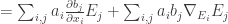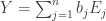$Y$ . What about in other bases? Well, assuming that $Y = \sum_{j=1}^n b_j E_j$ , we can just apply the product rule on the terms:

$\nabla_X Y = \sum_{i=1}^n a_i\nabla_{E_i} \sum_{j=1}^n b_j E_j$
$= \sum_{i=1}^n a_i \left(\sum_{j=1}^n \left(\nabla_{E_i} b_j\right) E_j + \sum_{j=1}^n b_j \nabla_{E_i} E_j\right)$
$= \sum_{i,j} a_i \frac{\partial b_j}{\partial x_i} E_j + \sum_{i,j} a_i b_j \nabla_{E_i} E_j$

In Cartesian coordinates, the second term is going to vanish, because the coordinate directions don’t change with respect to any direction. So our assumption about Cartesian coordinates is correct. In other bases, we can just think of the second term as a corrective factor for the curvature of the coordinate frames. In most texts, the vector $\nabla_{E_i} E_j = \sum_{k=1}^n \Gamma_{ij}^k E_k$ is defined, where the $\Gamma_{ij}^k$ are called Christoffel symbols. I won’t get into them here, except to say that they have some important symmetries.

Riemannian Connections

If you’re familiar with this material, you may have noticed that I’ve hand-waved a lot. There’s a lot of machinery that needs to be set up to prove existence and uniqueness of all these constructs. It’s also machinery that works fairly well in Euclidean space, but we can’t make the same assumptions on general smooth manifolds. We’d like a connection that works on general manifolds, but we need to make some extra assumptions. A Riemannian connection is an affine connection with some extra properties:

$\nabla_X Y - \nabla_Y X = \left[X,Y\right]$
$\nabla_X\left<U,V\right> = \left<\nabla_X U,V\right> + \left<U,\nabla_X V\right>$

Where $\left<\cdot,\cdot\right>$ is an inner product on the tangent space, and $\left[\cdot,\cdot\right]$ is the Lie bracket. The first condition imposes a restriction on the coordinate frames that states that the frames must be torsion-free; that is, the coordinate frames may not twist when moving in any particular direction. The second just imposes the product rule on the inner product. Euclidean space already has these properties, so the covariant derivative as I described it above is a Riemannian connection.

These extra rules basically allow us to assume that a connection $\nabla$ is unique on any particular smooth manifold that has an inner product defined on its tangent space, and that we can use the above formula to write it out explicitly. There’s a lot more to it, of course, but we have enough to work with. I’ll be writing more posts that cover this topic, but I encourage you to read up on it yourself and derive your own intuition of what’s going on.

2 Comments

Posted in Geometry, Topology

Tagged connection, covariant derivative, differential geometry basics, Riemannian

New Theme

Posted on May 28, 2009 | Leave a comment

Ugh. I hate the old theme’s treatment of images (a drop shadow under every image? Really?), so I’m using a new one. This one’s clean and simple, and handles the LaTeX just fine.

Leave a comment

Posted in Blog

Tagged theme

May Miscellany

Posted on May 2, 2009 | Leave a comment

It’s been a little while since I posted, so I thought I’d post some end-of-semester miscellaneous items.

I figured out my hangup about writing (with some help): I don’t know what the hell I’m doing. Your first reply may be to say, “well, duh!”, and you’d be right to say that. However, being new to something isn’t a feeling that I’m used to anymore. I’m coming out of a career where someone could hand me a project and I could get started with very few problems. Not so with research writing, as was pointed out to me.
I thought the fear angle was it for a while, but then I mulled it over, along with the comments people left in that vein. They were good observations, I think, but I’m not convinced that it’s fear. I’m a bit intimidated, don’t get me wrong, but I think that more than anything else I’m just lost. So, time for practice, practice, practice, and a little (ok, much) guidance from the people I write with.
Blip.fm: This is a pretty fun service. It’s kind of like Twitter, except every “blip” has a song mapped to it. The page has a built-in flash player so that you can listen to people’s (DJ’s) streams. I tried Pandora a while ago, and I picked it up again recently, and it just failed me. I can’t find the music that I like, and it always seems to bring in songs that don’t have the right sound for what I’m trying to get at.
Blip.fm is nice because you can just pick the songs, or scan around to find people listening to stuff that you like. There are certainly DJ’s on Blip.fm who try to get as many listeners as possible, but I just use it to store songs that I like or that I found cool at any particular moment. Here’s my stream if you’re interested. Like I said, it’s what I like, not what you like, so be forewarned.
It’s weird what’s useful: I was able to apply the core technique of an image-processing algorithm that I learned at my last job (not anything they patented, if they’re reading) to a class project this semester. I’ve discussed it with the postdoc interested in the technique, and it promises to be lots of fun. Even cooler is that the application is mostly unrelated to image processing (though it could be used in that capacity).

Leave a comment

Posted in Web, Writing

Tagged blip.fm, I'm a n00b

Why Do I Hate Writing Research Down?

Posted on April 24, 2009 | 18 comments

Obviously, I don’t hate all writing, or else I wouldn’t have a blog. It’s also not true when it comes to documentation because code documentation is one of the things that I try to do habitually and that I harped on all the time while I was an engineer. For some reason, though, I can’t motivate myself to write my research down, even though I view it as essential and essentially the same as code documentation. I need to pull my own teeth to start writing.

Even now, I’m experiencing an incredible stubbornness to just doing it. I have a deadline (not for a conference) to get something written down soon, which will serve to get some material written, but I would much rather be personally motivated to do it. If I want to do it, I’ll do it better. So I’m writing this out as an exercise to help me figure out why I’m being such an ass about it, to glean some advice from my readers, and maybe to help anyone else who is having trouble with a similar motivation.

When put on the spot, I could probably invent a couple inane excuses as to why I don’t want to write. They wouldn’t be accurate, however, because I really don’t know why. So here’s a few possibilities:

Procrastination: This is incredibly likely, but it’s outweighed by the fact that I still don’t want to write under my imminent deadline.
Pride: Also another possibility. I’m not denying it, since pride often accompanies (if not causes) stubbornness. But what would it be pride over? That I shouldn’t have to write? I’ve been aware since I chose this career change that writing will be an integral part of my work. Whither the pride, then?
Perfectionism: A strong candidate, but writing is an iterative process, and perfectionism undoes writing by dragging it out, not preventing it from starting.
Fear: Hmm. I think I might be getting somewhere. I don’t know where exactly it would stem from, but since I typed the word, it’s lingering there.

I’ll pause there for now, and I’ll go over some of the suggestions that people have already given me for motivation (all good):

It’s necessary anyway: I’ll have to write anyway, and I’ll have to revise a bunch of times, so there’s no point in putting it off.
It will help reveal flaws: I both agree and disagree with this. Mostly I agree, but it’s a good enough reason to just write it down.
It will help in communicating the research verbally: I really like this idea, and I’m eager to try it out. Now if I could just get over the hump…
Write every day: John suggested this in the comments to help overcome the inertia. The procrastinator in me dislikes this idea, but I think it’s important enough to try.

I want to work this out now, as early as possible, so that I’m not wasting so much time trying to motivate myself to write. The fear thing seems weird to me. Am I just having a fear of rejection or judgment? I thought I made this change ready to face both.

So, readers, any suggestions on motivations? How did (do) you get over the hump? Do you think it’s just some stupid fear of rejection/judgment? Or is it something else?

18 Comments

Posted in Writing

A Rant on Password Challenge Questions, If I May

Posted on April 5, 2009 | 6 comments

Fact: I select passwords that have a chasm separating them from my personal life. I use a system that only I know (not even my wife knows it), and I adhere to good password practices.

Fact: Personal data is researchable.

Ergo: Answers to personal questions are less secure than my passwords that they “protect.”

My bank doesn’t understand this crucial security notion:

Forcing me to use a system that is less secure than the one that I use now is a security flaw.

Incidentally, they also enforce passwords with a minimum number of a certain type of character, which is also less secure.

Security concerns aside, this is also an inconvenience. Passwords that I choose are cryptic, but I can commit them to memory. Security questions on the other hand, have “natural” answers. How forgiving will the verification be? If it’s lax, then it’s even less secure. If it’s strict, it’s a phenomenal inconvenience to me, because I might type the answer with a capital (or without), or use a numeral or abbreviation, etc. You get the idea. Now I’m stuck going to the branch just for fat-fingering something.

Security measures that are insecure and inconvenient aren’t worth it. Now, if someone could just convince the TSA of that…

[Update: An xkcd about the same topic the very day after I posted this:

Weird.]

6 Comments

Posted in Outside, Web

Tagged bank, rant, security, security theater

Afghanistan

Posted on April 2, 2009 | 1 comment

Whenever I see photos of Afghanistan, I’m always shocked at the geophysical resemblance of that country to my home state of Utah and to the neighboring state to the West, Nevada. The political resemblance is, of course, minimal. I hope that some day it can be just another beautiful place to see.

1 Comment

Posted in Outside

Tagged Afghanistan, photography, war

My Social Web Experiences

Posted on March 31, 2009 | Leave a comment

Well, since WoBloMo is officially a bust, I may as well not try to get posts in on time. It’s been an interesting exercise in posting regularly, and I have to say that it wasn’t all bad. I was surprised that I was able to come up with this many things to write about. This is one of those days when I’m at a loss, so I’ll just blab about my experiences with social media for a post.

Like most people, I didn’t see the point in the social web sites, like Facebook. I guess Twitter falls into that category too. I tried Twitter first, and I have to say that I didn’t see it. I didn’t know why people used it at all. Then I was on a mobile plan with unlimited texts, that no one took advantage of, so I decided to do something with them. I added Twitter to my mobile phone and that’s when I got it. For some reason, it’s incredibly entertaining to hear from various people about what they’re doing and what’s on their mind.

That last bit is what you have to realize about Twitter. When you can just blab about what’s on your mind and you don’t care what friends see it or who in the world sees it, and then someone that you didn’t know starts following you because they have something in common with you, that’s pretty cool. I cut off the unlimited texts because of my lifestyle change, so I had to get my Twitter fix somehow. I didn’t get TweetDeck the first time I tried it, but I tried it again, and I’m addicted. I follow lots more people now because of it. It’s a near necessity for following many people. If you follow me on Twitter, you know just how much I use it.

Facebook is kind of a different story for me. What was cool about Facebook was that I started getting in touch with all these people that I hadn’t talked to in years. That was also a downside, I might add. But it’s mostly a positive. For me, even keeping up with email correspondence seems difficult. But on Facebook, you can see what an acquaintance is up to right away, and then you remember to drop a note.

For me, I guess, Twitter and Facebook are kind of the same activity as writing letters was to my grandparents. Except it’s a lot faster, and suits my distracted nature.

Leave a comment

Posted in Web

Tagged Facebook, Twitter

WoBloMo: Fail

Posted on March 28, 2009 | Leave a comment

I forgot to post yesterday. And I was so close to the end of the month!

Oh well. If you’re at all curious about how my talk went (probably not) then I can tell you that it went well. I need some practice on a few things, like planning and time management, and Suresh pointed out that I write microscopically on the board. I also realized that I didn’t plan my board layout well enough, and I glossed over bits that would have really driven the message home.

As for the paper, it’s incredibly fascinating once you get into it. I recommend it to anyone interested in the bound on union find with path compression, and why the hell the inverse Ackermann function appears there.

Leave a comment

Posted in Blog, Presenting

Tagged path compression, woblomo

on Topology

Back in the Saddle

Geodesics

Straight Lines

The Exponential Map

Arc Length

Sources

Riemannian Connections

Covariant Derivatives of Scalar Functions

Covariant Derivatives of Vector Fields

Affine Connections

Riemannian Connections

New Theme

May Miscellany

Why Do I Hate Writing Research Down?

A Rant on Password Challenge Questions, If I May

Afghanistan

My Social Web Experiences

WoBloMo: Fail

Search It!

Recent Entries

Links